
Traffic flow theory is the scientific study of how vehicles move collectively on road networks, analysing the relationships between speed, flow, and density to explain, predict, and manage traffic behaviour. Rooted in physics and mathematics, it gives transport engineers the tools to diagnose congestion, design better infrastructure, and model the consequences of change before a single lane is built. The Greenshields model, the fundamental diagram, and the Lighthill-Whitham-Richards kinematic wave model are the three pillars every practitioner needs to understand. Whether you are a student encountering these concepts for the first time or a professional applying them daily, this guide covers the theory from first principles to real-world application.
What is traffic flow theory and why does it matter?
Traffic flow theory treats vehicles on a road network as a collective system rather than a collection of independent drivers. Traffic is modelled system-wide rather than as individual decisions, which is what makes it powerful. A single driver braking unexpectedly can trigger a shockwave that travels backwards through traffic for kilometres, even when the original cause has long since cleared. Understanding that mechanism is the foundation of the entire discipline.
The formal term used in transportation engineering is traffic flow theory, sometimes referred to as traffic flow analysis when the focus shifts from modelling to measurement and interpretation. Both terms describe the same body of knowledge. The distinction matters because practitioners often use analysis methods drawn directly from theoretical models, and conflating the two can lead to misapplied tools.

The importance of traffic flow theory extends well beyond academic interest. Theory guides data-driven operational improvements such as adding turn lanes, adjusting signal timing, and identifying where congestion will form under future demand. Without a theoretical framework, traffic engineering reduces to guesswork.
What are the fundamental variables and equations in traffic flow theory?
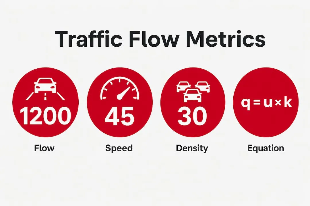
Three measurable variables define the state of any traffic stream: flow (q), speed (u), and density (k). Flow is the number of vehicles passing a fixed point per unit time, typically expressed in vehicles per hour. Speed is the space mean speed across a road section, measured in kilometres per hour. Density is the number of vehicles occupying a unit length of road, expressed in vehicles per kilometre or vehicles per mile per lane.
The relationship between these three variables is captured by the fundamental traffic flow equation: q = u × k. This single equation underpins virtually every traffic model in use today. If you know any two variables, you can calculate the third.
Typical variable ranges across traffic states
| Traffic state | Density (veh/mi/ln) | Speed (mph) | Flow (veh/hr/ln) |
|---|---|---|---|
| Free flow | Below 12 | Near free-flow speed | Low to moderate |
| Stable flow | 12–67 | Declining | Approaching capacity |
| Breakdown | Above 67 | Sharply reduced | Below capacity |
| Jam | 185–250 | Near zero | Near zero |
Free-flow density sits below 12 vehicles per mile per lane, while breakdown conditions begin above 67 vehicles per mile per lane. Jam density, the point at which traffic stops entirely, ranges from 185 to 250 vehicles per mile per lane. These thresholds are not arbitrary. They represent empirically observed transitions between distinct traffic regimes.
The Greenshields model adds a linear relationship between speed and density: as density increases from zero to jam density, speed decreases linearly from free-flow speed to zero. From this, maximum capacity is derived as qmax = uf × kj / 4, where uf is free-flow speed and kj is jam density. Capacity occurs at exactly half the free-flow speed and half the jam density. That result is elegant and practically useful for preliminary design calculations.
Pro Tip: When using the Greenshields model for capacity estimation, treat the result as an upper bound. Field data consistently show that actual capacity is lower because speed collapses more sharply near jam conditions than the linear model predicts.
How do traffic flow models characterise different traffic states?
The fundamental diagram is the standard graphical tool for representing traffic states. It plots the three paired relationships: flow against density, speed against density, and speed against flow. Each curve tells a different story about how a road section behaves as demand increases.
The Lighthill-Whitham-Richards model and shockwaves
The kinematic wave model, developed independently by Lighthill, Whitham, and Richards in the 1950s and known as the LWR model, treats traffic as a compressible fluid. It explains how disturbances propagate upstream as waves. A queue forming at a bottleneck does not stay fixed. It moves backwards through traffic at a speed determined by the slope of the fundamental diagram. This is why you can encounter stationary traffic on a motorway with no visible cause ahead.
Bottlenecks cause approximately 40% of all roadway congestion. That figure underscores why identifying and managing bottleneck locations is one of the highest-value activities in traffic engineering. The LWR model provides the mathematical basis for predicting where queues will form and how far they will extend.
Capacity drop and hysteresis
One of the most practically significant phenomena in traffic flow theory is the capacity drop, also called hysteresis. Once congestion forms at a bottleneck, the flow that the bottleneck can discharge drops by 5–10% below its pre-breakdown capacity. This means that clearing a queue is harder than preventing one. The road effectively becomes less efficient the moment it breaks down.
The Greenshields model, while mathematically convenient, underestimates speed drops near jam densities. Field data show a sharper, non-linear collapse of speed as density approaches jam conditions. More advanced models, including the Newell-Daganzo triangular fundamental diagram, better capture this behaviour and are preferred for operational analysis.
| Model | Assumptions | Best use case |
|---|---|---|
| Greenshields linear | Linear speed-density relationship | Preliminary capacity estimates |
| LWR kinematic wave | Traffic as compressible fluid | Queue propagation and shockwave analysis |
| Newell-Daganzo triangular | Two-regime linear approximation | Bottleneck and signal analysis |
| Microscopic car-following | Individual vehicle interactions | Detailed intersection or merge modelling |
Pro Tip: Never rely solely on the fundamental diagram from a single data source. Calibrate your model against site-specific loop detector or probe vehicle data, because capacity values vary significantly between road types, driver populations, and weather conditions.
What are the scales of traffic flow modelling?
Three modelling scales exist in traffic flow theory, each suited to different analytical problems.
-
Microscopic models simulate individual vehicles and their interactions. Car-following models such as the Intelligent Driver Model track each vehicle’s acceleration and deceleration in response to the vehicle ahead. These models are computationally intensive but capture detailed behaviour at junctions, merges, and weaving sections. Software packages like VISSIM and AIMSUN use microscopic simulation as their core engine.
-
Mesoscopic models represent vehicles in groups or platoons, using probabilistic distributions to describe their behaviour. They sit between microscopic detail and macroscopic simplicity, making them useful for corridor-level analysis where individual vehicle tracking is unnecessary but aggregate models are too coarse.
-
Macroscopic models treat traffic as a fluid, using aggregate variables of flow, speed, and density without tracking individual vehicles. The LWR model is the canonical macroscopic model. These models run quickly and are well suited to network-level strategic analysis and long-term planning.
Choosing the wrong scale is a common and costly mistake. Macroscopic models often fail to accurately predict delays at signalised intersections because signal control operates on individual vehicle arrivals and departures, not aggregate flows. Using a macroscopic model to evaluate junction signal timing will produce unreliable results. Microscopic simulation is the correct tool for that task.
How is traffic flow theory applied in transportation planning?
Traffic flow theory moves from academic framework to practical engineering through a structured sequence of analysis steps.
-
Data collection. Loop detectors, radar sensors, Bluetooth readers, and GPS probe data provide the raw measurements of flow, speed, and occupancy. Modern intelligent transport systems (ITS) deliver this data in real time, enabling dynamic traffic management.
-
Bottleneck identification. By plotting observed flow and density against the fundamental diagram, engineers locate where a road section is operating near or above its capacity. Traffic flow analysis identifies congestion hotspots and quantifies the severity of each bottleneck.
-
Model calibration. Theoretical models are fitted to site-specific data. Free-flow speed, jam density, and capacity are estimated from observations rather than assumed from textbook values.
-
Scenario testing. Calibrated models are used to test interventions before implementation. Adding a lane, changing a signal plan, or introducing a variable speed limit can each be evaluated against the fundamental diagram or within a simulation environment.
-
Infrastructure and policy decisions. Results feed directly into design standards and operational strategies. Practical traffic engineering integrates theory with the Highway Capacity Manual, accounting for factors such as heavy vehicle composition, pedestrian crossings, and environmental conditions.
The Highway Capacity Manual, published by the Transportation Research Board in the United States and widely referenced internationally, codifies traffic flow principles into level-of-service assessments. It translates theoretical variables into practical grades from A (free flow) to F (breakdown), giving planners a common language for communicating road performance.
Key takeaways
Traffic flow theory is the essential analytical framework connecting measurable road conditions to engineering decisions, and no transport professional can apply it effectively without understanding the fundamental diagram, model scale selection, and the capacity drop phenomenon.
| Point | Details |
|---|---|
| Core equation | The relationship q = u × k links flow, speed, and density and underpins every traffic model. |
| Capacity drop | Once congestion forms, bottleneck capacity falls by 5–10%, making prevention more effective than recovery. |
| Model scale matters | Macroscopic models suit network planning; microscopic models are required for junction and signal analysis. |
| Bottleneck significance | Bottlenecks cause approximately 40% of all congestion, making their identification a priority task. |
| Theory meets practice | The Highway Capacity Manual translates traffic flow principles into level-of-service grades used in real design decisions. |
Why I think traffic flow theory is underused in practice
Most transport engineers I have spoken with over the years can recite the fundamental equation. Far fewer apply it rigorously when making real decisions. There is a persistent tendency to reach for simulation software without first checking whether the underlying model is calibrated to local conditions. A VISSIM model built on default parameters is not a traffic flow analysis. It is an expensive way to confirm your assumptions.
The Greenshields model is taught early and remembered fondly because it is mathematically tidy. But field data show a sharper collapse of speed near jam conditions than the linear model predicts, and engineers who forget that will consistently overestimate capacity. The gap between textbook theory and field behaviour is where most planning errors originate.
The most exciting development in the field right now is the integration of real-time GPS probe data with classical macroscopic models. Connected vehicle data and ITS sensors are giving practitioners access to continuous, network-wide observations that were simply not available when the LWR model was published. The theory has not changed. The quality of the data feeding it has transformed what is possible.
My advice to students is to spend time with real detector data before you spend time with simulation software. Plot your own fundamental diagrams from loop detector records. Find the capacity drop in the data. That experience will make every model you build afterwards more grounded and more credible.
— Rob
Build your career in traffic and transport engineering

Traffic flow theory sits at the heart of highways engineering, traffic management, and transportation planning. Professionals who can apply traffic flow models, interpret fundamental diagrams, and translate analysis into infrastructure decisions are in consistent demand across the UK and internationally. Jobs-in-transport has connected transport professionals with specialist roles since 2005, covering everything from traffic signal engineering to strategic transport planning. If you are ready to apply your knowledge of traffic flow principles in a professional setting, browse current vacancies across highways, traffic management, and transport technology on the platform today.
FAQ
What is the fundamental equation in traffic flow theory?
The fundamental equation is q = u × k, where q is flow in vehicles per hour, u is space mean speed, and k is density in vehicles per unit length. Every traffic flow model is built on this relationship.
What causes capacity drop at a bottleneck?
Capacity drop, also called hysteresis, occurs when congestion forms at a bottleneck and reduces its discharge flow by 5–10% below the pre-breakdown level. This means a congested road operates less efficiently than the same road before breakdown occurred.
What is the difference between microscopic and macroscopic traffic models?
Microscopic models simulate individual vehicles and their interactions, making them suitable for junction and signal analysis. Macroscopic models treat traffic as a fluid using aggregate variables, making them better suited to network-level and strategic planning.
How is traffic flow analysis used in infrastructure planning?
Traffic flow analysis identifies bottlenecks, quantifies congestion severity, and tests interventions such as lane additions or signal timing changes before they are built. Results are assessed against frameworks like the Highway Capacity Manual to inform design decisions.
What is the Greenshields model and where does it fall short?
The Greenshields model assumes a linear relationship between speed and density, from which maximum capacity is derived as qmax = uf × kj / 4. Its limitation is that it underestimates how sharply speed collapses near jam density, so it tends to overestimate capacity under high-demand conditions.


